728x90
반응형

-------------- FATAL CALLED ---------------

FATAL CALLED FROM FILE:  <stdin>  LINE:     930

 ... Could not find matching time in input file wrfchemi_d01_2016-05-02_00:00:00

-------------------------------------------

application called MPI_Abort(MPI_COMM_WORLD, 1) - process 0


Sol>


namelist.input auxinput5_interval_m = 360 라인을 comment out 시킨다. 라인이 존재하면, 동일한 wrfchemi_d01_2016-05-02_00:00:00 파일에서 6시간 간격의  emission 시간을 찾는다. 없애면 default 파일 마다 매시간 데이터를 불러온다.


  • VPRM input 읽을 문제
728x90
반응형
728x90
반응형


해결


http://forum.wrfforum.com/viewtopic.php?f=10&t=347

WRF 매뉴얼 5-14의 Real Data Cases 읽어보라.


해결>>> SET input_from_file = T for each domain !!!!

728x90
반응형
728x90
반응형

Wrfchemi_ d01 d02 모두 링크 되어 있음

&time_control

input_from_file                     = .true.,.true.,

/

&bdy_control

specified                           = .true., .true.,

nested                              = .false.,.false.,

/

&chem

chem_opt                            = 16,      16,

chemdt                              = 30,      30,

chem_conv_tr                        = 0,       0,

chem_in_opt                         = 1,       1,

have_bcs_chem                       = .true.,  .true.,

kemit                               = 1,

io_style_emissions                  = 2,

emiss_opt                           = 16,      16,

emiss_inpt_opt                      = 16,      16,

bio_emiss_opt                       = 0,       0,

bioemdt                             = 30,      30,

phot_opt                            = 0,       0,

photdt                              = 30,      30,

depo_fact                           = 0.25,    0.25

gas_bc_opt                          = 0,       0,

gas_ic_opt                          = 0,       0,

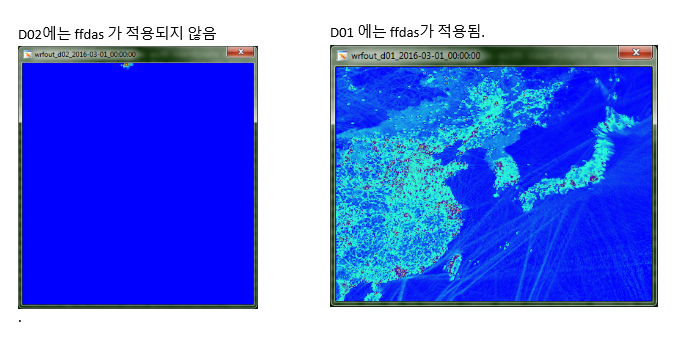
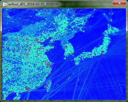
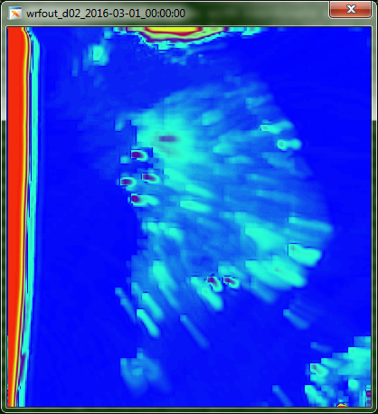
D01 에는 ffdas 적용됨.

한반도 농도가 너무 낮다.  한자리수…

서쪽 bc 380

.

&time_control

input_from_file                     = .true.,.true.,

/

&bdy_control

specified                           = .true., .true.,

nested                              = .false.,.false.,

/

&chem

chem_opt                            = 16,      16,

chemdt                              = 30,      30,

chem_conv_tr                        = 0,       0,

chem_in_opt                         = 1,       1,

have_bcs_chem                       = .true.,  .false.,

kemit                               = 1,

io_style_emissions                  = 2,

emiss_opt                           = 16,      16,

emiss_inpt_opt                      = 16,      16,

bio_emiss_opt                       = 0,       0,

bioemdt                             = 30,      30,

phot_opt                            = 0,       0,

photdt                              = 30,      30,

depo_fact                           = 0.25,    0.25

gas_bc_opt                          = 0,       0,

gas_ic_opt                          = 0,       0,


해결


&time_control

input_from_file                     = .true.,.false.,

/

&bdy_control

specified                           = .true., .false.,

nested                              = .false.,.true.,

/

&chem

chem_opt                            = 16,      16,

chemdt                              = 30,      30,

chem_conv_tr                        = 0,       0,

chem_in_opt                         = 1,       1,

have_bcs_chem                       = .true.,  .false.,

kemit                               = 1,

io_style_emissions                  = 2,

emiss_opt                           = 16,      16,

emiss_inpt_opt                      = 16,      16,

bio_emiss_opt                       = 0,       0,

bioemdt                             = 30,      30,

phot_opt                            = 0,       0,

photdt                              = 30,      30,

depo_fact                           = 0.25,    0.25

gas_bc_opt                          = 0,       0,

gas_ic_opt                          = 0,       0,


728x90
반응형
728x90
반응형

Registry.EM_COMMON


Wrf391


# Variables from WPS

#


state    real   u_gc           igj      dyn_em      1        XZ    i1  "UU"     "x-wind component"    "m s-1"

state    real   v_gc           igj      dyn_em      1        YZ    i1  "VV"     "y-wind component"    "m s-1"


# lsm State Variables

state    real   VEGFRA           ij     misc        1         -     i024rhd=(interp_mask_field:lu_index,iswater)u=(copy_fcnm)   "VEGFRA"           "VEGETATION FRACTION" ""


# Velocities

#

# U Vel

state    real   u              ikjb     dyn_em      2         X     \

     i0rhusdf=(bdy_interp:dt)       "U"                      "x-wind component"   "m s-1"

state    real   ru             ikj     dyn_em      1         X      -        "MU_U"        "mu-coupled u"   "Pa m s-1"


registry.chem


# Additional variables for CO2 and GHG options

# The following variables are to run the VPRM model; The vegfra_vprm is for VPRM only and it's different than VEGFRA in wrfinput

state   real     -               i{ghgv}jf    vprm_in     -        -     -          -              "VPRM input fields"                  ""

state   real   vegfra_vprm       i{ghgv}jf    vprm_in     1        -     i{15}rh  "VEGFRA_VPRM"    " " " "

state   real   evi               i{ghgv}jf    vprm_in     1        -     i{15}rh  "EVI"            " " " "

state   real   evi_min           i{ghgv}jf    vprm_in     1        -     i{15}rh  "EVI_MIN"         " " " "

state   real   evi_max           i{ghgv}jf    vprm_in     1        -     i{15}rh  "EVI_MAX"         " " " "

state   real   lswi              i{ghgv}jf    vprm_in     1        -     i{15}rh  "LSWI"           " " " "

state   real   lswi_max          i{ghgv}jf    vprm_in     1        -     i{15}rh  "LSWI_MAX"        " " " "

state   real   lswi_min          i{ghgv}jf    vprm_in     1        -     i{15}rh  "LSWI_MIN"        " " " "

728x90
반응형
728x90
반응형

1) Set up the analysis nudging fdda namelist. Carefully read test/em_real/README.namelist file to understand the meaning of each namelist variable in the FDDA section, which is also listed below:

grid_fdda (max_dom) Analysis nudging switch (1=on, 0=off) for each domain. The 3D analyses must be provided here in model horizontal and vertical coordinate space. Note that the nudging coefficient (e.g., guy, gt, gq) is used to effectively turn on or off analysis nudging for each variable. For example, gt must be set to 0.0 to turn off analysis nudging for 3D temperature if grid_fdda = 1 for a given domain.
gfdda_inname Analysis nudging input file name defined in Real
gfdda_interval_m (max_dom) Time interval (min) between analysis times. For example, set this parameter to 360 if you are using 6-hourly analyses.
gfdda_end_h (max_dom) Time (h) after model start time for last analysis used for 3D analyses nudging. For example, set this parameter to 24 if you are using 3D analyses ending at 24 h after initial time of forecast.
io_form_gfdda Analysis data io format (2=netCDF)
fgdt (max_dom) Calculation frequency (minutes) for analysis nudging (0=every step). We suggest you use this default value.
if_no_pbl_nudging_uv (max_dom) A switch to control nudging of u-component and v-component of wind in vertical (0=nudging of u and v in the PBL, 1=no nudging in the PBL). This switch is similar to INONBL(1) and INONBL(2) in MM5.
if_no_pbl_nudging_t (max_dom) A switch to control nudging of temperature in vertical (0=nudging of temp in the PBL, 1=no nudging in the PBL). This switch is similar to ININBL(3) in MM5.
if_no_pbl_nudging_q (max_dom) A switch to control nudging of water vapor mixing ratio (q) in vertical (0=nudging of q in the PBL, 1=no nudging of q in the PBL). This switch is similar to ININBL(4) in MM5.
if_zfac_uv (max_dom) A switch to control nudging of u-component and v-component of wind in vertical (0=nudge ua and v for all layers, 1=limit nudging to levels above or larger than k_zfac_uv). For example, model level 1 is always at the surface and say model level 15 is at 850 mb for your case, and below this level you wish to turn analysis nudging off for wind. You would ten set this parameter to 1 and the following parameter to 15.
k_zfac_uv (max_dom) Model level below which nudging is switched off for u and v.
if_zfac_t (max_dom) A switch to control nudging of temperature in vertical (0=nudge temperature for all layers, 1=limit nudging to levels above k_zfac_t).
k_zfac_t (max_dom) Model level below which nudging is switched off for temperature.
if_zfac_q (max_dom) A switch to control nudging of water vapor mixing ratio in vertical (0=nudge temperature for all layers, 1=limit nudging to levels above k_zfac_q).
k_zfac_q (max_dom) Model level below which nudging is switched off for q.
guv (max_dom) Nudging coefficient for u and v (sec-1)
gt (max_dom) Nudging coefficient for pot. temperature (sec-1)
gq (max_dom) Nudging coefficient for water vapor mixing ratio (sec-1)
if_ramping A switch to decide if nudging is ramped down linearly (0=nudging ends abruptly as a step function, 1=ramping nudging down linearly at end of period.
dtramp_min Duration of ramping down (min). Its sign determines how the ramping is done (60.0=ramping starts at last analysis time, -60.0=ramping ends at last analysis time).


Since analysis nudging works for multiple domains within the same job, some of the namelist variables are defined in multiple columns, so that the user can choose a specific domain to apply analysis nudging. The following is an example that involves three domains in the same job, using 3D analysis nudging:


&fdda

grid_fdda =       1, 1, 1,

gfdda_inname =       "wrffdda_d",

gfdda_end_h =        24, 24, 24,

gfdda_interval_m =       360, 360, 360,

fgdt =        0, 0, 0,

if_no_pbl_nudging_uv =       0, 0, 0,

if_no_pbl_nudging_t =       1, 1, 1, 

if_no_pbl_nudging_q =       1, 1, 1, 

if_zfac_uv =       1, 1, 1, 

k_zfac_uv =       10, 10, 10, 

if_zfac_t =       0, 0, 0, 

k_zfac_t =       10, 10, 10, 

if_zfac_q =       0, 0, 0, 

k_zfac_q       10, 10, 10, 

guv =       0.0003, 0.0003, 0.0003, 

gt =       0.0003, 0.0003, 0.0003, 

gq =       0.0003, 0.0003, 0.0003, 

if_ramping =       1,

dtramp_min =       60.0, 

io_form_gfdda =       2, 

/


2) Run real using the above namelist which is also used in WRF in the next step. When namelist variables grid_fdda, gfdda_end_h, and gfdda_interval_m are properly set, run real.exe to create FDDA input files (e.g., wrffdda_d01, wrffdda_d02, etc. if max_dom > 1). This example indicates that Real will create analysis files for all three domains (if max_dom = 3), and the format of the FDDA file is in NETCDF (i.e., io_form_gfdda = 2). The last analysis time is 24 hours, and the analysis interval is 6 hours. The rest of the namelist variables are not required for program Real.


3) Run WRF after the above namelist has been defined properly. For example, the above namelist indicates that analysis nudging is turned on for all three domains, with identical nudging coefficients for u, v, theta, and q for all three domains, but within the PBL the analysis nudging for temperature and moisture fields are turned off for all three domains. Note that nudging for each variable is controlled by the nudging coefficient value. It is not recommended that nudging after a pre-forecast period be abruptly turned off since this can create noise, so the example also indicates that analysis nudging is ramped down for a period of 60 minutes, starting from hour 24 and ending at hour 25. Analysis nudging is completely turned off at hour 25. The example further indicates that analsyis nudging for wind is turned off with the 'zfac' option within the lowest 10 model layers for all three domains, regardless of the if_no_pbl_nudging_uv switch. If both zfac and if_no_pbl_nudging_uv are turned on, nudging will be set to zero through at least the lowest 10 vertical layers, and higher if the PBL height is larger than the height of the 10th model layer above the surface.


The equations and further details of analysis nudging can be found in Stauffer and Seaman (1990) and Stauffer et al. (1991). The latter paper introduces surface analysis nudging, which can take advantage of higher temporal resolution gridded surface analyses (e.g., hourly or 3-hourly) than the 3D analyses (e.g., 6-hourly or 12-hourly), and the former are applied within the model diagnosed PBL. This separate capability for higher temporal resolution surface analysis nudging will be avaialable in a future release of WRF. Some typical applications of analysis nudging as part of a muti-scale FDDA strategy, including observation nudging, can be found in Stauffer and Seaman (1994), Seaman et al. (1995), Stauffer et al. (2000), Tanrilulu et al. (2000), Otte et al. (2001), Leidner et al. (2001), Deng et al. (2004), Deng and Stauffer (2006), and many others.


REFERENCES:


Deng, A. N. L. Seaman, G. K. Hunter, and D. R. Stauffer, 2004: Evaluation of inter-regional transport using the MM5/SCIPUFF system. J. Appl. Meteor., 43, 1864-1886.


Deng, A., and D. R. Stauffer, 2006: On improving 4-km mesoscale model simulations. J. Appl. Meteor. and Climat., 45, 361-381.


Leidner, S. M., D. R. Stauffer, and N. L. Seaman, 2001: Improving California coastal zone numerical weather prediction by dynamic initialization of the marine layer. Mon. Wea. Rev., 129, 275-294.


Otte, T. L., N. L. Seaman, and D. R. Stauffer, 2001: A heuristic study on the importance of anisotropic error distributions in data assimilation. Mon. Wea. Rev., 129, 766-783.


Seaman, N. L, D. R. Stauffer, and A. M. Lario-Gibbs, 1995: A multi-scale four-dimensional data assimilation system applied in the San Joaquin Valley during SARMAP: Part I: Modeling design and basic performance characteristics. J. Appl. Meteor., 34, 1739-1761.


Stauffer, D. R., and N. L. Seaman, 1990: Use of four-dimensional data assimilation in a limited-area mesoscale model. Part I: Experiments with synoptic-scale data. Mon. Wea. Rev., 118, 1250-1277.


Stauffer, D. R., N. L. Seaman, and F. S. Binkowski, 1991: Use of four-dimensional data assimilation in a limited-area mesoscale model. Part II: Effects of data ssimilation within the planetary boundary layer. Mon. Wea. Rev., 119, 734-754.


Stauffer, D. R., and N. L. Seaman, 1994: On multi-scale four-dimensional data assimilation. J. Appl. Meteor., 33, 416-434. 


Tanrikulu, S., D. R. Stauffer, N. L. Seaman, and A. J. Ranzieri, 2000: A field-coherence technique for meteorological field-program design for air-quality studies. Part II: Evaluation in the San Joaquin Valley. J. Appl. Meteor., 39, 317-334.

728x90
반응형
728x90
반응형
  1. 먼저, surface upper OBS 데이터를 합친다. 3시간 간격으로


cat ./surface/SURFACE_OBS:2016050100 ./upper/OBS:2016050100 > ./OBS:2016-05-01_00

cat ./surface/SURFACE_OBS:2016050106 ./upper/OBS:2016050106 > ./OBS:2016-05-01_06

cat ./surface/SURFACE_OBS:2016050112 ./upper/OBS:2016050112 > ./OBS:2016-05-01_12

cat ./surface/SURFACE_OBS:2016050118 ./upper/OBS:2016050118 > ./OBS:2016-05-01_18

cat ./surface/SURFACE_OBS:2016050200 ./upper/OBS:2016050200 > ./OBS:2016-05-02_00

cat ./surface/SURFACE_OBS:2016050206 ./upper/OBS:2016050206 > ./OBS:2016-05-02_06

cat ./surface/SURFACE_OBS:2016050212 ./upper/OBS:2016050212 > ./OBS:2016-05-02_12

cat ./surface/SURFACE_OBS:2016050218 ./upper/OBS:2016050218 > ./OBS:2016-05-02_18


$ cd /data1/chpark/little_R/2010.calnex

$ ./concat

 This script combine surface and upper observation to one file for each 6-h obs data


  1. Confirm all OBS: 05-13 to 06-17.


  1. $ cd ~/OBSGRID


  1. 위에서 작성된 3시간 간격 데이터를 하나로 합친다.


  1. $ edit namelist.oa

(1) namelist.oa 내에서 /data1/chpark/little_R/2010.calnex/OBS 설정해 줘야 된다.

(2) Change data and time frame

(3) domain 3 대해서만.


  1. $ ln -sf WPS/met_em.d03* .


  1. ./obsgrid.exe

*** 주의: OBS_DOMAIN3XX  에서 100개가 넘어가면, running 하지만, OBS_DOMAIN 작성되지 않는다. 따라서 12일씩 끊어서 돌려야.


  1. ./concat_all script 사용해서, OBS_DOMAIN301 파일로 통합한다.


  1. ./em_real OBS_DOMAIN301 copy 두면, namelist.input 에서 obs nudging option 따라 불러온다.
728x90
반응형
728x90
반응형

Feng's wrfchemi_d03 

  1. 단위: (mol km^-2 hr^-1)/10**4
  2. /일은 morning rush hour peaks 없다.
  3. 문제점: 요일이 맞다.

시작을 2011 5 1 () 설정. 사실 2010 51 () 해야 .


Vulcan wrfinput_d03 (plus 3day 1hr)

  1. Feng's emission 비교하면서, Vulcan / 피크를 찾음.

일요일: 오전 피크 없음.

토요일: 이른 아침 작은 피크 (금요일 야간 활동 영향)


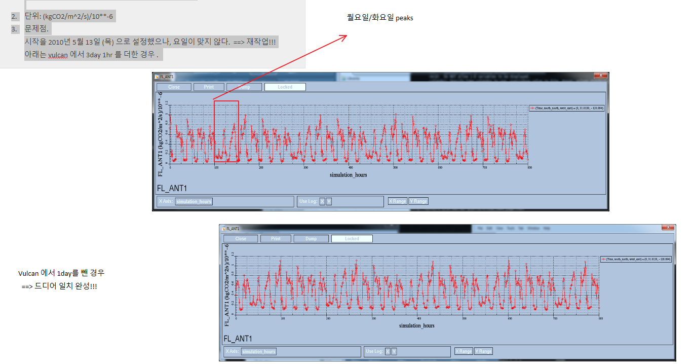
  1. 단위: (kgCO2/m^2/s)/10**-6
  2. 문제점.

시작을 2010 5 13 () 으로 설정했으나, 요일이 맞지 않다.  ==> 재작업!!!

아래는 vulcan 에서 3day 1hr 더한 경우 .


With Feng's Hestia emission data

  1. Hestia E_CO2 (Unit: mol km^-2 hr^-1)/10**4)


LA 도심: 4-13

항구 근처: 6-7

SE 포인트 근처: 0-1


  1. Original Hestia from Gerney (Unit: KgC km^-2 hr^-1)
728x90
반응형
728x90
반응형
  • 관측데이터 획득

http://rda.ucar.edu/datasets/ds351.0    : upper air BUFR format

                                                     /ds461.0   : sfc BUFR format

                                                     /ds608.0   : NARR


Saved at

~/data/little_R/upper/OBS:*

                           /surface/SURFCAE_OBS:*


  • Concat_upper.sfc script 파일로 파일 합치고, 이름 바꾸기

$ cat .upper/OBS_   ./surface/SURFACE_OBS    > ./OBS_ 


  • ./obsgrid.exe 실행하면,

Plotobs_out_d0X

Qc_obs_raw.

Qc_obs_used

Metoa_em.                                    : 초기장이 met_em 에서 바뀜

OBS_DOMAIN330                         : 1-hr 마다 output 바뀜

Wrfsfdda_d03                           : 요건 하나만 나오고, 6hr 마다 바뀜  ==> version 3.1 이상에서 사용 가능 wrfsfdda     


등등이 나온다


  • OBS_DOMAIN3XX   등은 concat_OBS_DOOMAIN  으로 합치고 real.exe 진행한다.
728x90
반응형
728x90
반응형

자료

  1. Goes SST

6 km (0.05 x 0.05 ) ; 1, 3, 24 h 자료 있음.


http://podaac.jpl.nasa.gov/dataset/GOES_L3_SST_6km_NRT_SST_24HOUR


  1. RTG SST


0.083 8~9 km. 6시간 간격


ftp://polar.ncep.noaa.gov/pub/history/sst/ophi


  1. OISST version 2 AVHRR SST

Daily SST data (0.25 x 0.25 ); 24시간 간격


https://iridl.ldeo.columbia.edu/SOURCES/.NOAA/.NCDC/.OISST/.version2/.AVHRR/.sst/


https://www.ncdc.noaa.gov/thredds/oisst-catalog.html


방법

  1. Download the SST file from

ftp://polar.ncep.noaa.gov/pub/history/sst/ophi


  1. Unzip rtg_sst_grb_hr_0.083.200808.gz


  1. Do geogrid.exe

Edit namelist.wps

$ ./geogrid.exe


  1. Do ungrib.exe  for NARR_3D and NARR_SFC

Edit namelist.wps

$ ln -sf ./ungrib/Variable_Tables/Vtable.NARR ./Vtable

$ ./link_grib.csh NARR_3D

GRIBFILE 확인

$ ./ungrib.exe

Edit namelist.wps

$ ./link_grib.csh NARR_SFC

GRIBFILE 확인

$ ./ungrib.exe


  1. Do ungrib.exe for SST

Edit namelist.wps

$ ln -sf ./ungrib/Variable_Tables/Vtable.SST ./Vtable

$ ./link_grib.sh SST

GRIBFILE 확인  *******중요

$ ./ungrib.exe


  1. Do metgrid.exe

Edit namelist.wps

Fg_name = 'NARR_3D', 'NARR_SFC', 'SST'     ****** 3개를 한꺼번에 metgrid.exe 해야 .


  1. Confirm that there is SST variable in met_em files.


  1. > ./real.exe     실행후,  wrflowinp_d0X 파일 생성하는지 확인!


  1. Edit namelist.input

Io_form_auxinput4     =  2

Auxinput4_inname     = "wrflowinp_d<domain>" (creadted by real.exe)

Auxinput4_interval     = 360,   360,   360,

728x90
반응형
728x90
반응형

http://www2.mmm.ucar.edu/wrf/OnLineTutorial/DATA/NARR/index.html  ==> 요것만 참고하면 된다.


자료:

https://rda.ucar.edu/#!lfd?nb=y&b=proj&v=NCEP North American Regional Reanalysis


NARR Data

As the start and end dates are the same,

interval_seconds will be ignored.

NARR (North American Regional Reanalysis) data.

Type: GRIB1 data

Resolution:

Area - approx. 160E–20W ; 10N–80N ; at 32 km

Output frequency 3 hourly

29 pressure levels (1000-100hPa ; excluding surface)

Availability:

January 1979 to current

From NCAR/RDA site at: http://rda.ucar.edu/pub/narr/ (You must register -it is free- to access the data.)


Download the 3D, flx and sfc files for the date of interest. (Follow the links to this data from the left-hand panel on the above web site.)

The downloaded files will have the following file names:

merged_AWIP32.YYYYMMDDHH.3D

merged_AWIP32.YYYYMMDDHH.RS.flx

merged_AWIP32.YYYYMMDDHH.RS.sfc

Also download (you only need to do this once), the FIXED file. This file contains the fields, LANDSEA; SOILHGT; SOIL_CAT and VEGCAT. The date stamp in this file is 1979-11-08_00. (Follow the "NARR Fixed Fields" link from the left-hand panel on the above web site, and then download the "32km output GRIB file".)


Vtable: Vtable.NARR


  Peruse the ungib/Variable_Tables/Vtable.NARR file to see which fields we are going to try and unpack from the GRIB files. This file also contains notes regarding which fields are obtain from which of the above files.
There is a problem with the supplied Vtable (see post in Known Problems dated 3/15/07). Please download a new version and place it the ungib/Variable_Tables/ directory.


Sample data (December 2006):

The data is available for the period 2006-02-05_12 to 2006-02-06_12 (data frequency is 3 hourly).

This is GRIB 1 data.

Notes on running UNGRIB for this data

1. Download data and place in directory ../DATA/NARR

2. Examine the GRIB files, (as an example we will look at a surface file, but also examine the other files)

   ./util/g1print.exe ../DATA/NARR/merged_AWIP32.2006020512.RS.sfc

3. ln -sf ungrib/Variable_Tables/Vtable.NARR Vtable


4a. ./link_grib.csh ../DATA/NARR/rr-fixed.grb

5a. Edit namelist.wps

    start_date = '1979-11-08_00:00:00',

    end_date = '1979-11-08_00:00:00',

    interval_seconds = 10800,

    prefix = 'NARRFIX',

6a. ./ungrib.exe >& ungrib_data.log


4b. ./link_grib.csh ../DATA/NARR/merged_AWIP32.200602

      The above command will link in all the 3D, flx and sfc data files for the time of interest,

      so that we can work with them as a single dataset.

5b. Edit namelist.wps

    start_date = '2006-02-05_12:00:00',

    end_date = '2006-02-06_12:00:00',

    interval_seconds = 10800,

    prefix = 'NARR',

6b. ./ungrib.exe >& ungrib_data.log


7. Examine the intermediate files, e.g.,

   ./util/rd_intermediate.exe NARRFIX:1979-11-08_00

   ./util/plotfmt.exe NARRFIX:1979-11-08_00 ; idt gmeta


  You only have to do steps 4a-6a once, even is you change to a different case date, as this is a fixed file.
Steps 4b-6b must be repeated for each new case date.


Notes on running METGRID for this data

Since we have change the 'prefix', in the namelist, ensure that you set 'fg_name' correct before running metgrid.exe

fg_name = 'NARR'

We also have some constant fields we need to input into the met_em* files. To do this ADD, the following line to the metgrid section of the namelist:

constants_name = './NARRFIX:1979-11-08_00'


Pasted from <http://www2.mmm.ucar.edu/wrf/OnLineTutorial/DATA/NARR/index.html>


  1. 체크할 사항

Met_em. 파일에 num_metgrid_soil_level = 4 인지 확인할 .

728x90
반응형

+ Recent posts